simdata: A package for creating simulated datasets

Introduction

Simulation studies in statistics or other methodological research fields are controlled experiments used to assess the properties of algorithms, gauge the performance of statistical or machine learning models, and gain insights into complex phenomena which are not readily understood analytically. While simulation studies by nature are simplifying the “true” underlying mechanisms of interest, they are useful because they allow the complete specification of the “ground truth” to which comparisons can be made and the experimental conditions are fully under control of the experimenter. This is in contrast to data obtained from observational studies, in which many factors may influence the resulting measurements.

Simulation studies typically consist of three major components:

A data generating mechanism
The methods or models to be evaluated
Evaluation criteria to assess the methods after application to the generated data

All three together make up what we will call the simulation study design.

The data generating mechanism usually simulates (i.e. creates) data according to pre-defined parameters, e.g. the number of variables (i.e. columns of the data matrix) to be generated, their correlation structure or the number of observations (i.e. rows of the data matrix). Usually, the data generation involves some uncertainty or noise when creating the data, to mimic the uncertainty when data is obtained through measurements in the real world or sampled from a population. Therefore, each simulation scenario can be conducted repeatedly to remove the effect of sampling variability.

The methods or models to be evaluated in the study are then applied to the datasets generated by the data generating mechanism and the evaluation criteria are computed, e.g. some measure of deviation from the ground truth.

Data generation with this package

The goal of the simdata package is to provide a simple yet flexible framework which supports the first step of a simulation study, namely the data generating mechanism.

The way data is created in this package involves the following procedure:

Draw an initial dataset Z from some probability distribution. An example might be to draw a number of variables with given correlation structure from a multivariate Normal distribution.
The initial data is then transformed via user specified transformation functions into the final dataset X. Examples for transformations could be to derive binary variables from Normal random variables or to change location and scale of the initial random variables.
The final dataset is optionally post-processed. Examples are to truncate the dataset to prevent problematic outliers or to standardize the data.

After these steps, the final dataset X can be used in the further steps of the simulation study.

Workflow with this package

In order to implement the outlined data generating mechanism, the user first has to define a simulation design. This is done by extending the S3 class simdesign, or using one of the pre-defined simulation designs, which is used to as an interface for further package functions. It stores all necessary information to generate data following the given specification. The actual data generation then happens in the simulate_data function. Please see the numerous examples below to quickly familiarize yourself with the package functionality.

Packages used

This vignette makes use of the tidyverse environment of packages and specifically requires the dplyr, purrr, ggplot2, forcats and GGally packages to be available, as well as the reshape2 package for data transformation. Furthermore, for the parallelization example the doParallel and doRNG package are loaded. Please refer to the R environment used to create this vignette for detailed information. In this vignette we will prefix all relevant function calls by :: to show the package which implements the function - this is not necessary but only done for demonstration purposes.

Example 1: Independent data, no transformation

We demonstrate a very basic example here:

Setup a design to sample from 5 independent normal variables
- Define a diagonal 5 x 5 correlation matrix (correlation_matrix)
- Ensure that the data is returned as a data.frame by passing the data.frame constructor to transform_initial. (Otherwise the data would be returned as a matrix.)
- Pass a prefix to the function to construct variable names
Simulate from the design to obtain 100 observations (n_obs) with a given random seed (seed).
Inspect the simulated data.

correlation_matrix = diag(1, nrow = 5)

sim_design = simdata::simdesign_mvtnorm(relations = correlation_matrix, 
                                        transform_initial = data.frame,
                                        prefix_final = "variable")
sim_data = simdata::simulate_data(sim_design, n_obs = 100, seed = 25897165)

knitr::kable(head(sim_data))

variable1	variable2	variable3	variable4	variable5
-0.4083281	1.3494810	0.6183227	-0.5885417	0.9910670
-1.3882168	-1.3453283	-0.8755803	-0.2168642	-2.3119306
-0.9298047	-0.2462345	0.1028683	-0.5223406	-0.4701425
1.3110934	-1.0087735	-0.6052583	2.0218711	0.8146569
-1.2179351	-0.8560356	-2.6381571	-0.0863500	0.3438921
0.3504726	-0.1930905	-1.0631527	-1.0101591	0.6001550

p = GGally::ggpairs(sim_data, 
                    upper = list(continuous = "points"), 
                    progress = FALSE) +
  theme_bw()
print(p)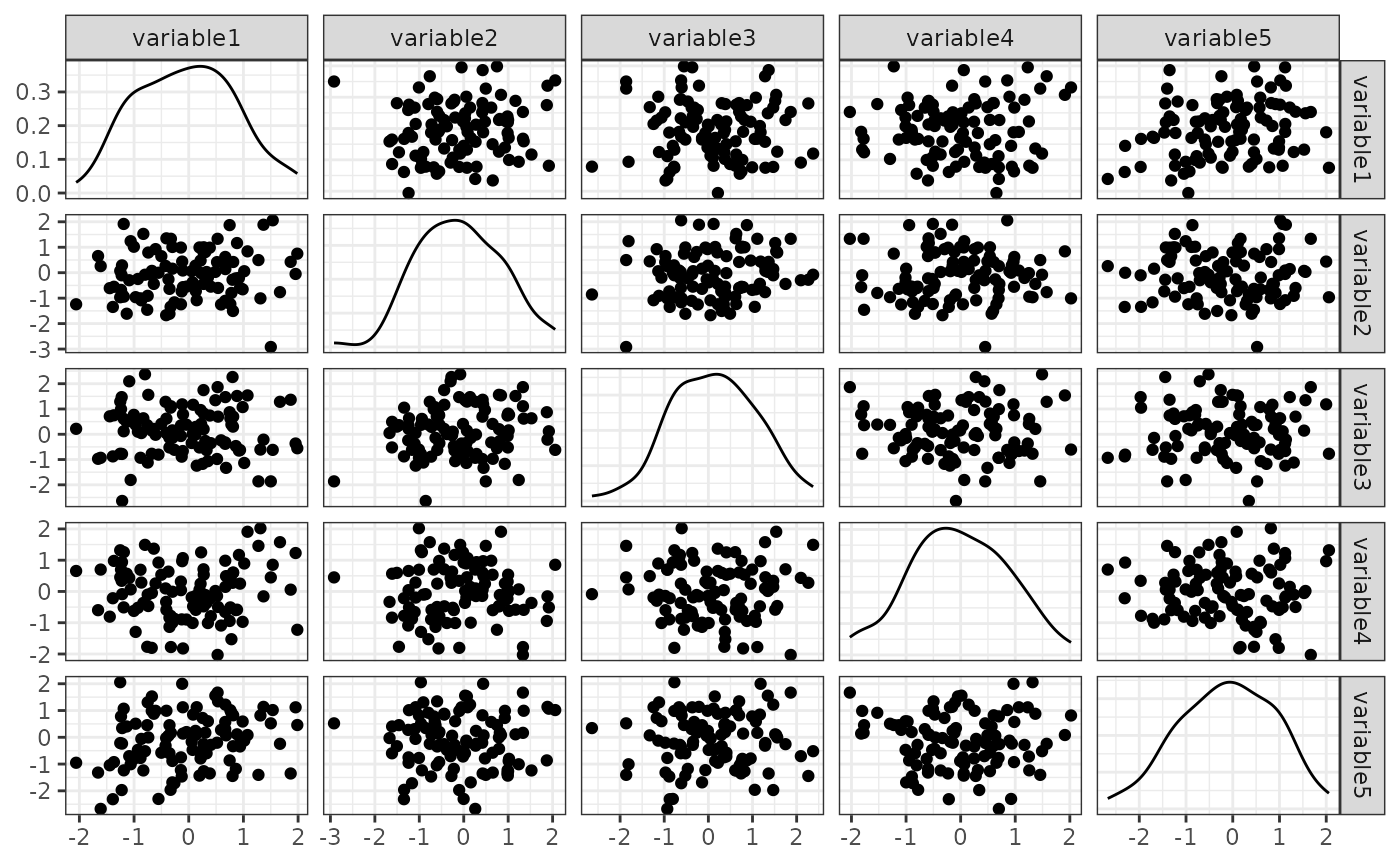

Example 2: Independent data, with transformation

In this example we transform the initial data to obtain a more interesting dataset. The basic principle follows Example 1.

Create a transformation function transformation using simdata::function_list
- Pass functions that transform the columns of the simulated, initial dataset as named arguments
- The number of columns in the final dataset is given by the number of transformations passed here
- To let the names of the arguments determine the final columnnames, set prefix_final to NULL in the simdesign constructor
Pass the created transformation function as transform_initial argument to the simdesign constructor.

correlation_matrix = diag(1, nrow = 5)
transformation = simdata::function_list(
  "v1" = function(x) x[, 1],
  "v2*2" = function(x) x[, 2] * 2, 
  "v3^2" = function(x) x[, 3]^2,
  "v4+v5" = function(x) x[, 4] + x[, 5], 
  check.names = FALSE # pass columnnames exactly as specified here
)

sim_design = simdata::simdesign_mvtnorm(
  relations = correlation_matrix,
  transform_initial = transformation, 
  prefix_final = NULL
)
sim_data = simdata::simulate_data(sim_design, n_obs = 100, seed = 25897165)

knitr::kable(head(sim_data))

v1	v2*2	v3^2	v4+v5
-0.4083281	2.6989619	0.3823229	0.4025253
-1.3882168	-2.6906566	0.7666409	-2.5287948
-0.9298047	-0.4924690	0.0105819	-0.9924831
1.3110934	-2.0175470	0.3663376	2.8365280
-1.2179351	-1.7120713	6.9598728	0.2575421
0.3504726	-0.3861811	1.1302936	-0.4100041

p = GGally::ggpairs(sim_data, upper = list(continuous = "points"), 
                    progress = FALSE) +
  theme_bw()
print(p)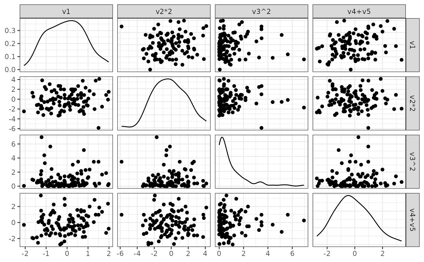

Example 3: Realistic, complex data

In this example we implement a design following Binder, Sauerbrei, and Royston (2011). The simulated data resembles data obtained from a biomedical study with a complex correlation pattern and different variable distributions.

Create a complex initial correlation matrix comfortably using simdata::cor_from_upper
- This defines the initial distribution as a multivariate Normal distribution Z with 15 dimensions
Use a variety of transformations to create numeric, binary and ordinal variables
- Using the transformation the initial distribution Z is transformed to the final dataset X with 17 columns

correlation_matrix = simdata::cor_from_upper(
  15, 
  rbind(c(1,2,0.8), c(1,9,0.3), 
        c(3,5,0.3), c(3,9,-0.5), 
        c(4,6,-0.5), c(4,7,-0.3),
        c(5,6,-0.3), c(5,12,0.5),
        c(6,7,0.5), c(6,11,0.5), c(6,14,0.3),
        c(7,11,0.3), c(7,14,0.3),
        c(8,9,-0.3), c(8,11,0.3),
        c(11,14,0.5)))

transformation = simdata::function_list(
  v1 = function(z) floor(10 * z[,1] + 55), 
  v2 = function(z) z[,2] < 0.6, 
  v3 = function(z) exp(0.4 * z[,3] + 3),
  v4 = function(z) z[,4] >= -1.2,
  v5 = function(z) z[,4] >= 0.75,
  v6 = function(z) exp(0.5 * z[,5] + 1.5),
  v7 = function(z) floor(pmax(0, 100 * exp(z[,6]) - 20)),
  v8 = function(z) floor(pmax(0, 80 * exp(z[,7]) - 20)),
  v9 = function(z) z[,8] < -0.35,
  v10 = function(z) (z[,9] >= 0.5) & (z[,9] < 1.5),
  v11 = function(z) z[,9] >= 1.5,
  v12 = function(z) 0.01*floor(100 * (z[,10] + 4)^2),
  v13 = function(z) floor(10 * z[,11] + 55),
  v14 = function(z) floor(10 * z[,12] + 55),
  v15 = function(z) floor(10 * z[,13] + 55),
  v16 = function(z) z[,14] < 0,
  v17 = function(z) z[,15] < 0
)

sim_design = simdata::simdesign_mvtnorm(
  relations = correlation_matrix,
  transform_initial = transformation,
  prefix_final = NULL
)

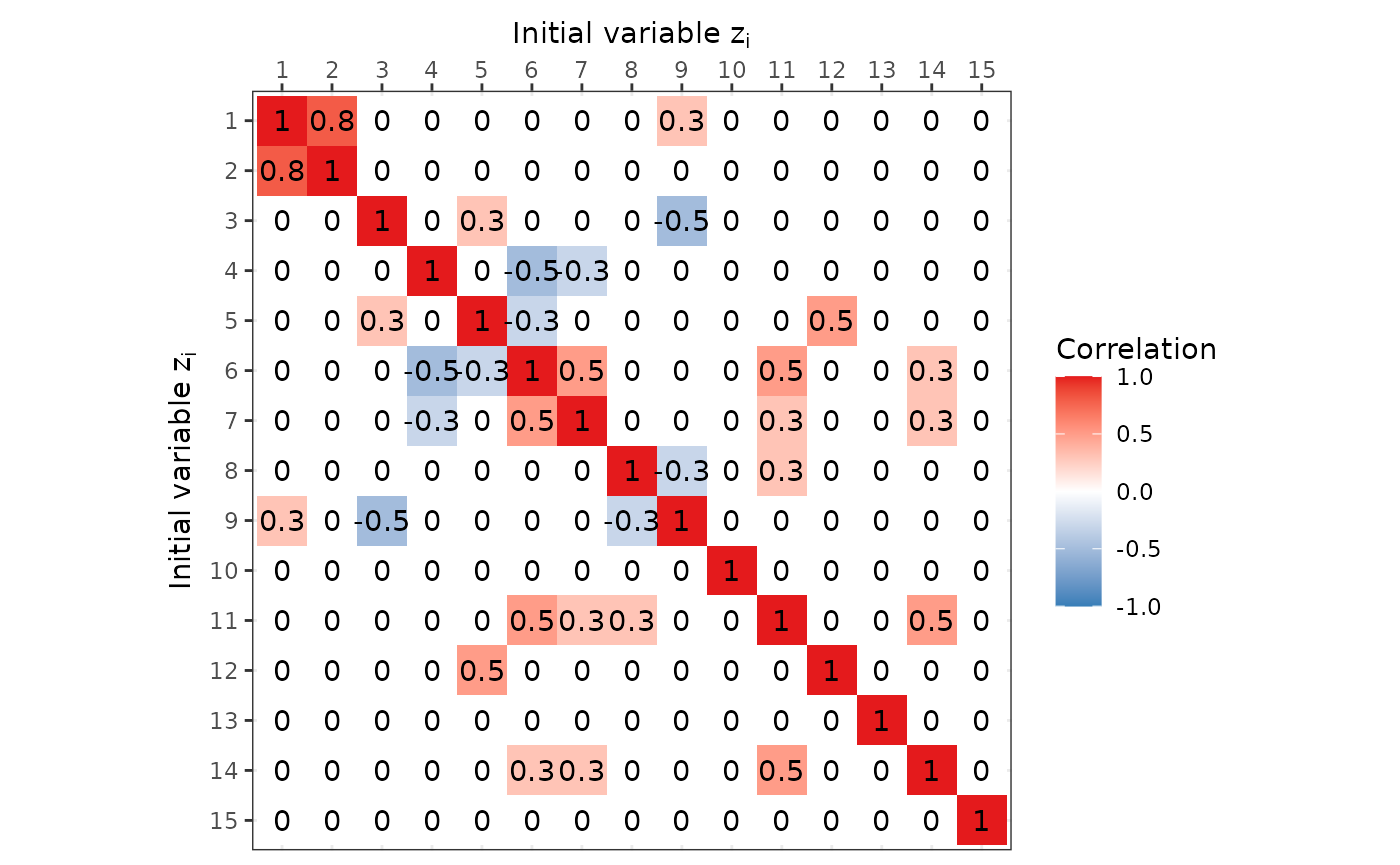
Visualisation of initial correlation matrix

We can display the correlation matrix of the initial underlying distribution using ggplot2. Or we can use the graph plotting tools from this package to display a basic correlation network.

Or we can use the simple graph visualisation provided by this package. To keep this graph simple, correlations below a certain threshold are removed. The simdata::plot_cor_network function provides several options to improve display of the graph, some of which are explained in more detail below. Here we just point out that the layout of the network is based on the Fruchterman-Reingold algorithm as implemented in the igraph package and therefore comprises random parts. Therefore, using a seed for the random number generation is advised.

simdata::plot_cor_network(sim_design, seed = 1)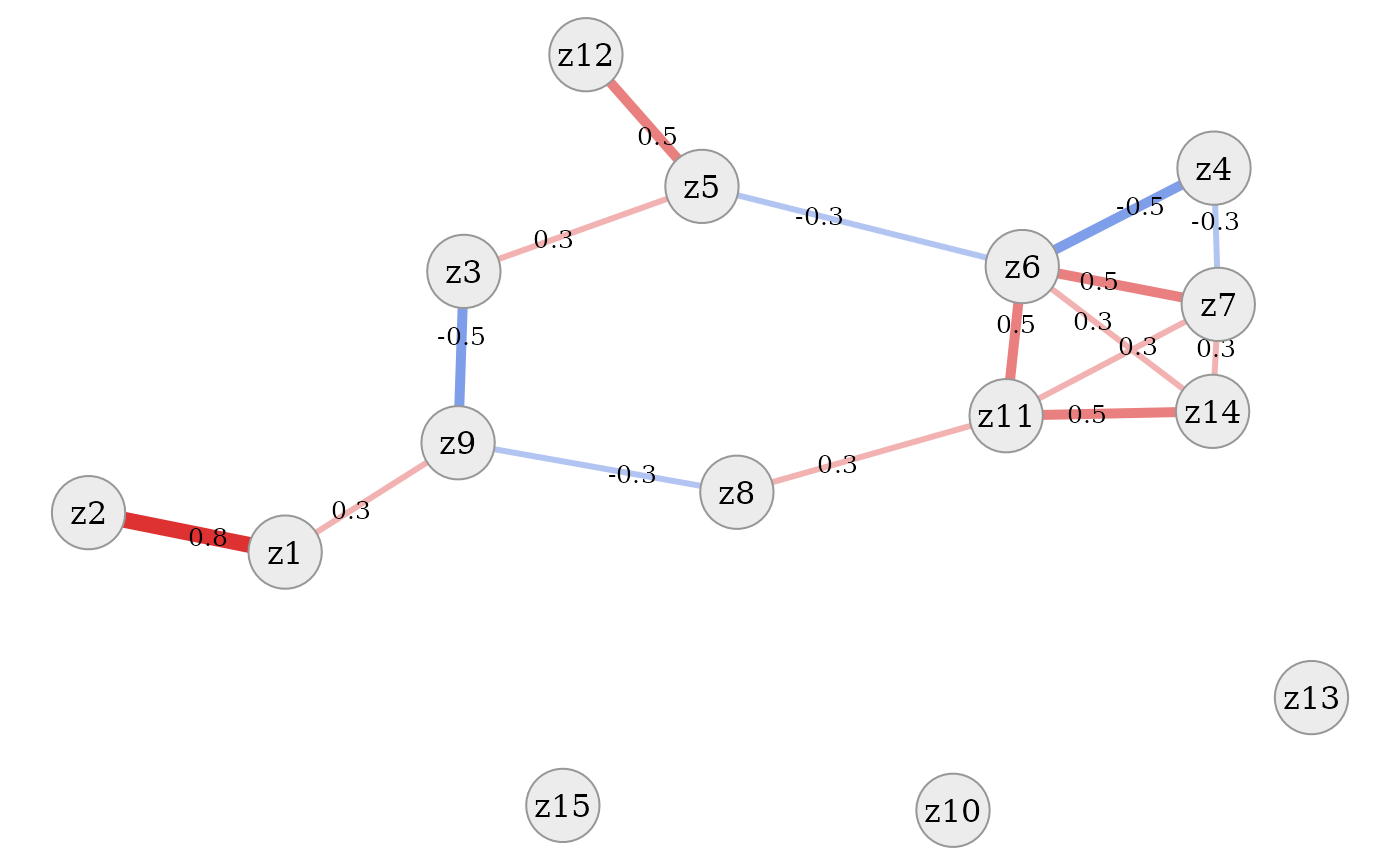

Simulation and visualisation of final data

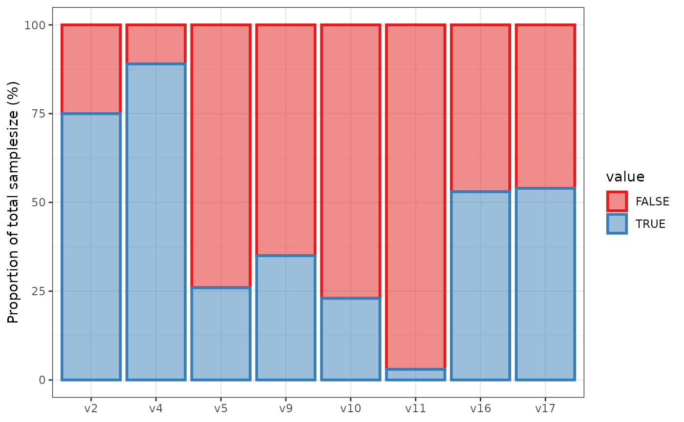
We simulate from the design and visualise numeric variables via violinplots and discrete variables via barplots using ggplot2.

sim_data = simdata::simulate_data(sim_design, n_obs = 100, seed = 25897165)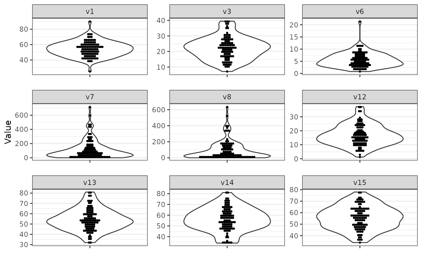

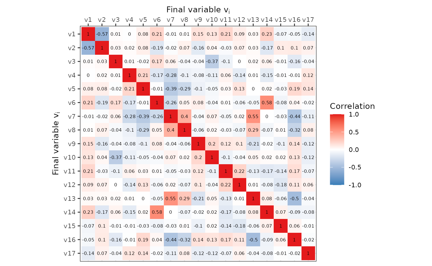
We can also plot the correlation structure of the single, final dataset via the correlation matrix and visualise it using ggplot2 or as a network using the functions provided by this package.

Visualisation of estimated correlation network

Note that the above correlation matrix is based on a single simulated dataset of a fixed size. To provide a robust and stable estimate of the correlation after transforming the initial dataset, one can employ approximation by simulation, as the initial correlation structure is affected by the data transformation and can not be analytically expressed in all cases. This can conveniently be achieved using estimate_final_correlation. The resulting correlation network can be visualized via plot_cor_network or by plot_estimated_cor_network which combines the estimation of the correlation matrix and the network plotting into one wrapper function.

Note that the layout algorithm of igraph computes a similar layout for initial and final correlation structure, given some manual tweaking of the random seed. This probably does not hold for all setups, but if the initial and final layout are somewhat similar (i.e. after proper pruning via cutting of low correlations), the resulting graphs may reflect that.

We demonstrate some basic plotting functionality (the arguments are identical for plot_cor_network):

Draw all edges in the graph by setting cor_cutoff to NULL
Turn off edge labeling by setting edge_label_function to NULL
Controling edge width using edge_width_function
Using edge weights (i.e. correlation between two variables) to influence the graph layout via use_edge_weights - higher edge weight brings vertices closer together

# draw full network
simdata::plot_estimated_cor_network(sim_design, 
                                    cor_cutoff = NULL, 
                                    edge_label_function = NULL,
                                    edge_width_function = function(x) x*25,
                                    use_edge_weights = TRUE, 
                                    edge.color = "clipped-ramp",
                                    seed = 2321673)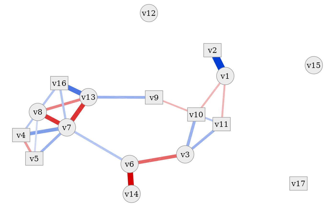

The following graphs all use the default correlation cutoff of 0.1.

Switching correlation type to Spearman using cor_type
- Note that when edge weights are used, then the networks for different correlation types can not be compared directly, as the vertex layout may change
Setting various other parameters
- Note the usage of mar to set the image margins to make the axes visisble
- Note that distinction between categorical and numeric data is turned off (show_categorical)

# simplify by using cor_cutoff
simdata::plot_estimated_cor_network(sim_design, 
                                    seed = 2)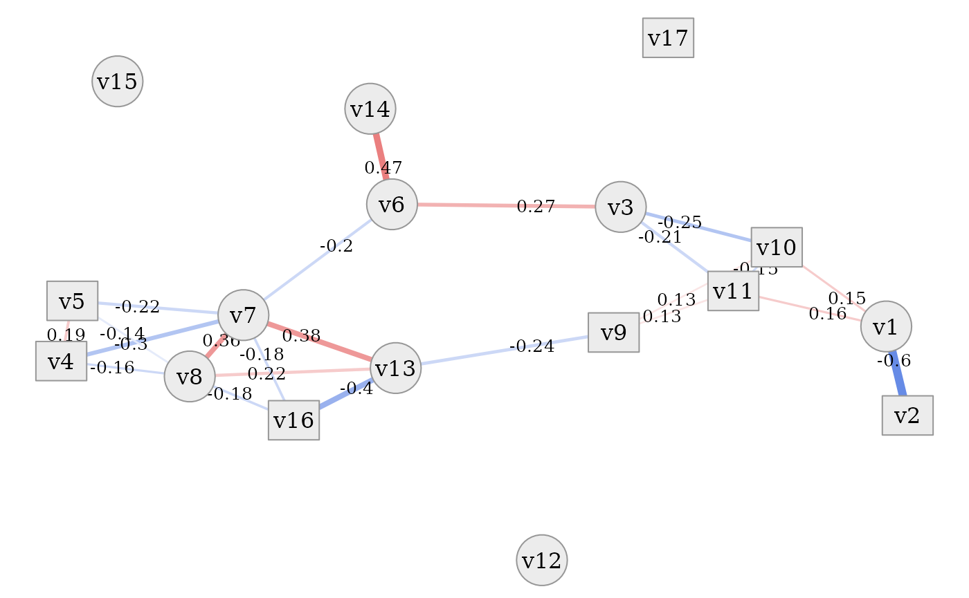

# set correlation type
simdata::plot_estimated_cor_network(sim_design, 
                                    cor_type = "spearman", 
                                    seed = 2321673)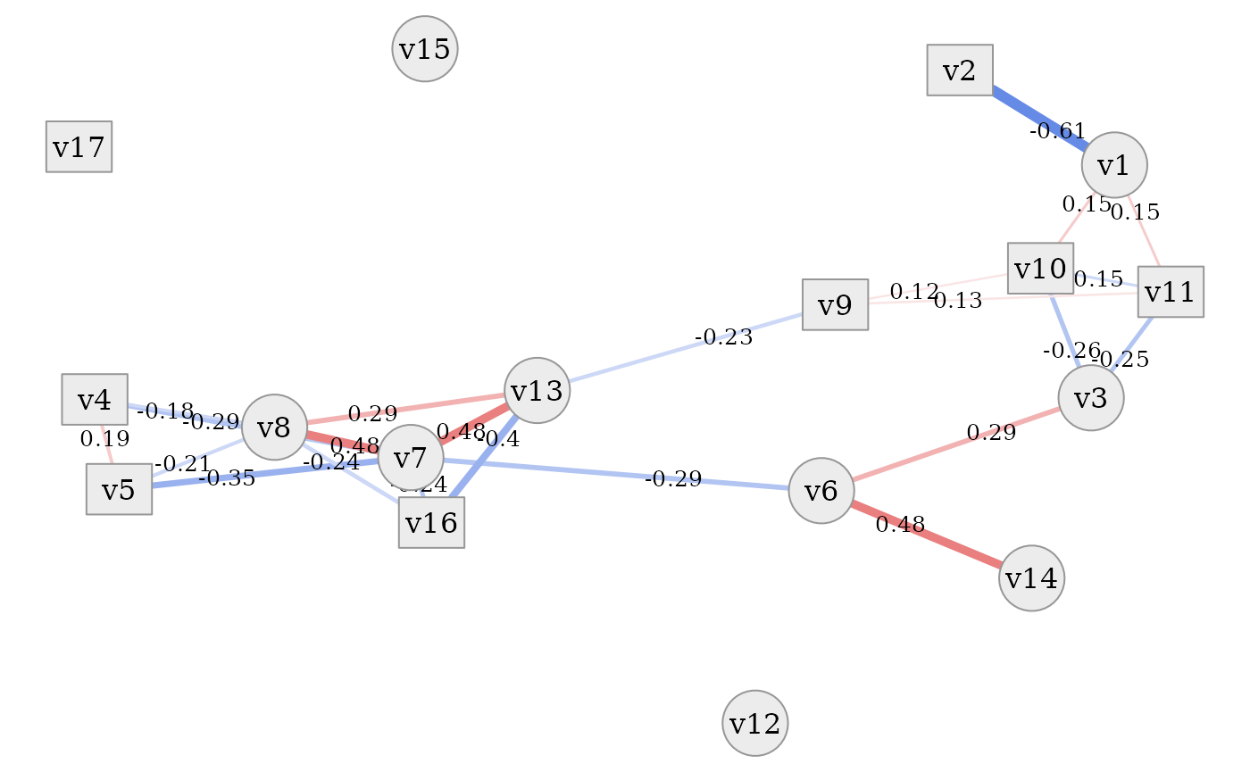

# set various parameters
simdata::plot_estimated_cor_network(sim_design, seed = 2321673, 
                                    edge.color = "red-blue", 
                                    axes = TRUE, cor_type = "s", 
                                    edge_width_function = function(x) var(x)*200,
                                    show_categorical = FALSE, 
                                    mar = c(2, 2, 0, 0))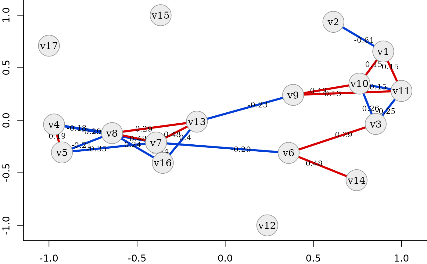

In all of these plots it is evident that the dataset contains a tight cluster of highly correlated variables (especially v4, v5, v7, v8, v13, v16) but also quite independent variables (v12, v15, v17). Some are also only connected to the network via one other variable (v2, v14). Thanks to the network layout of the plot, which is often more intelligible than a plain correlation matrix, this quite clearly shows the rich variety of correlation patterns within the simulated data.

Post-processing

Post-processing can be used to apply a number of functions to the dataset before it is returned by simulate_data. This is useful to e.g. standardize and truncate data, as shown below.

To add post-processing functions to the simdesign object, simply pass a list to the constructor or add it directly to the object. Each entry has a name (name of a function) and is a list with named arguments passed to the function (if default parameters should be used simply pass an empty list). See the do_processing help for further details. The simulation of the data does not need to be changed in any way.

Truncation

Add truncation to the post-processing via process_truncate_by_iqr
- Truncation is only added for specific numeric variables by passing a named vector

sim_design$process_final = list(
    process_truncate_by_iqr = list(
        truncate_multipliers = c(v6 = 2, v7 = 2, v8 = 2)
    )
)

sim_data = simdata::simulate_data(sim_design, n_obs = 100, seed = 25897165)

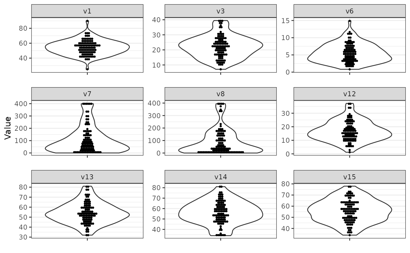
Compare the results with the results before and note the truncation in the specified variables (v6, v7, v8).

Note that the above truncation is based on statistics derived from each individual simulated dataset. To implement truncation based on statistics derived from the data generating mechanism itself, one can 1) simulate a reasonably large, untruncated dataset, 2) derive the desired upper and lower truncation thresholds, and 3) add process_truncate_by_threshold with the derived truncation thresholds to the simulator object to truncate by fixed tresholds in every simulation run. Truncation can be done independently for lower and upper thresholds (see example below).

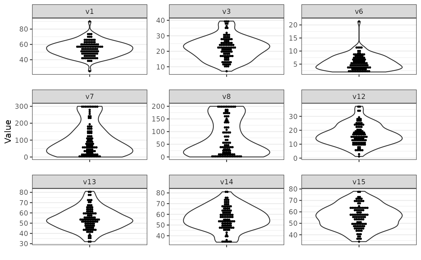
sim_design$process_final = list(
    process_truncate_by_threshold = list(
        truncate_upper = c(v8 = 200, v7 = 300),
        truncate_lower = c(v6 = 2)
    )
)

sim_data = simdata::simulate_data(sim_design, n_obs = 100, seed = 25897165)

Compare the results with the results before and note the truncation in the specified variables (v6, v7, v8).

Standardization

Similarly, standardization can be applied using the standard scale function, changing the scale on the y-axis of the following plots. Note that the order of functions passed via process_final is important. Since base::scale() returns a matrix, we also want to transform the result back to a data.frame in the end.

sim_design$process_final = list(
    process_truncate_by_iqr = list(
        truncate_multipliers = c(v6 = 2, v7 = 2, v8 = 2)
    ), 
    scale = list(), 
    data.frame = list()
)

sim_data = simdata::simulate_data(sim_design, n_obs = 100, seed = 25897165)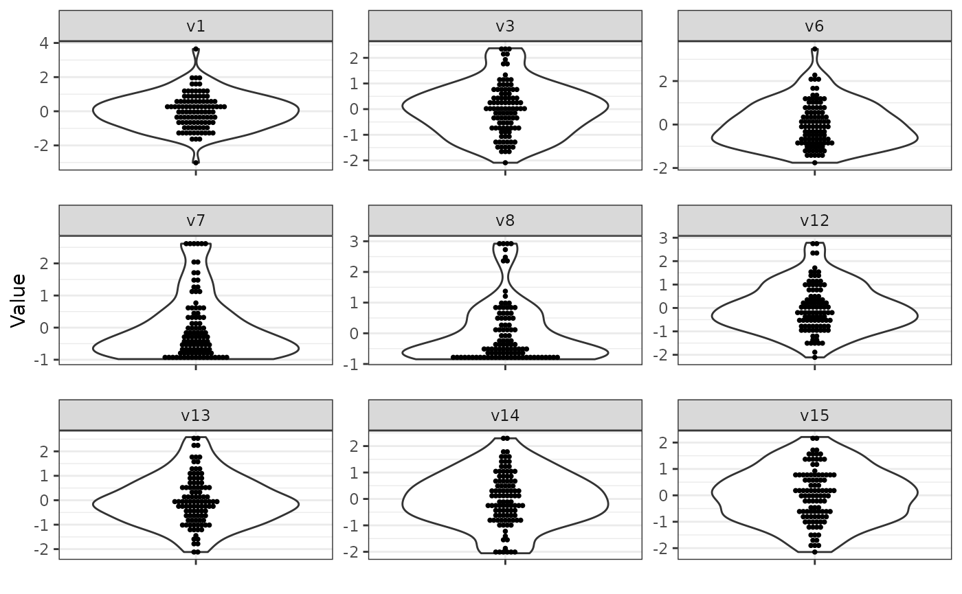

Advanced simulation setup

In the following we briefly present some more advanced usage aspects of the package.

Rejection sampling

A very simple form of rejection sampling is implemented in the simulate_data_conditional function, which only accepts a final dataset if it fulfills some specified conditions. This can be useful to prevent issues during simulation runs when the simulated data is e.g. likely to produce collinear matrices due to high dependencies between the variables or if some of them produce low variance variables.

Note that such an approach can lead to serious bias in the simulations if the rejection rate is very high. Thus, it might be necessary to revise such a setup or at least record the number of rejections for reporting purposes (as facilitated by the return_tries option of the function).

Usually rejections should occur very rarely. In this case the simulate_data_conditional function can be used to let the simulation run smoothly or let the calling function decide on how to handle rejections.

To show an example, we set up a very simple simulation with two variables and make them collinear on purpose via a transformation.

The is_collinear function from this package is used to check for collinearity
After at most three runs with rejected datasets the function returns (reject_max_iter)
The number of tries is returned in a list (return_tries)

correlation_matrix = diag(1, nrow = 2)
transformation = simdata::function_list("v1" = function(x) x[, 1],
                                        "v1*2" = function(x) x[, 1] * 2, 
                                        check.names = FALSE)

sim_design = simdata::simdesign_mvtnorm(
  relations = correlation_matrix,        
  transform_initial = transformation, 
  prefix_final = NULL
)

# ignoring the collinearity
sim_data = simdata::simulate_data(sim_design, n_obs = 100, seed = 2)
knitr::kable(cor(sim_data))

	v1	v1*2
v1	1	1
v1*2	1	1

# rejecting collinear matrices
sim_data = simdata::simulate_data_conditional(sim_design,
                                              n_obs = 100, seed = 2,
                                              reject = is_collinear,
                                              reject_max_iter = 3,
                                              return_tries = TRUE)

## Warning in reject(x): is_collinear: Matrix is not full rank.
## Warning in reject(x): is_collinear: Matrix is not full rank.
## Warning in reject(x): is_collinear: Matrix is not full rank.

## Warning in simdata::simulate_data_conditional(sim_design, n_obs = 100, seed = 2, : No suitable datamatrix found within iteration limit. Returning NULL.

sim_data

## $x
## NULL
## 
## $n_tries
## [1] 3

Note that multiple conditions can be checked by passing a function_list as rejection function. All of them must be fulfilled or the matrix is rejected.

In our example below we randomly transform the columns to be collinear or constant. However, in the end we obtain a result which passes both checks.

correlation_matrix = diag(1, nrow = 3)
transformation = simdata::function_list(
  "v1" = function(x) x[, 1],
  "might_be_collinear" = function(x) {
    if (rbinom(1, 1, 0.5)) {
      return(x[, 1] * 2)
    } else return(x[, 2])
  }, 
  "might_be_constant" = function(x) {
    if (rbinom(1, 1, 0.5)) {
      return(0)
    } else return(x[, 3])
  },
  check.names = FALSE)

sim_design = simdata::simdesign_mvtnorm(
  relations = correlation_matrix,        
  transform_initial = transformation,
  prefix_final = NULL
)

sim_data = simdata::simulate_data_conditional(
  sim_design,
  n_obs = 100, seed = 3,
  reject = simdata::function_list(is_collinear, 
                                  contains_constant),
  reject_max_iter = 3, 
  return_tries = TRUE)

## Warning in f(x): is_collinear: Matrix is not full rank.

## Warning in f(x): contains_constant: Matrix contains constant column.

## Warning in f(x): is_collinear: Matrix is not full rank.

sprintf("Number of tries: %d", sim_data[[2]])

## [1] "Number of tries: 3"

knitr::kable(head(sim_data[[1]]))

v1	might_be_collinear	might_be_constant
-1.5696270	1.4666759	-1.4960854
-1.1502890	-2.0230091	-0.6816524
0.5070104	0.7471119	0.1759890
-0.4375236	0.9427262	0.8910450
-1.6917860	-0.7121474	-0.3322689
0.9830335	-0.9880418	0.2655464

User defined `simdesign` classes

Other initial distributions

In this package, simulating initial data from a multivariate Normal distribution is already implemented in the simdesign_mvtnorm S3 class. However, it is easy to implement other distributions and extend the underlying interface of the simdesign class. To do this, all that needs to be implemented is the generator object of the new simulation class. Below we show how to code a toy wrapper to simulate binary data using the stats::rbinom function.

A new class must implement a generator function which takes one argument (number of observations to simulate) and outputs a two-dimensional array (matrix or data.frame)
A new class should always use ... to pass further arguments to simdesign
A new class should extend the class attribute to facilitate writing S3 methods which recognize the newly implemented class

binomial_simdesign <- function(size = 1, prob = 0.5, ...) {
  
  # define generator function
  # make sure it returns a two-dimensional array
  generator = function(n) matrix(rbinom(n, size = size, prob = prob), ncol = 1)
  
  # setup simdesign object
  # make sure to pass generator function and ...
  # all other information passed is optional
  dsgn = simdata::simdesign(
    generator = generator, 
    size = size, 
    prob = prob,
    ...
  )
  
  # extend the class attribute 
  class(dsgn) = c("binomial_simdesign", class(dsgn))
  
  # return the object
  dsgn
}

Finally, we can use the newly created class as in the examples before.

sim_design = binomial_simdesign(size = 1, prob = 0.7)
sim_data = simdata::simulate_data(sim_design, 100, seed = 1)
knitr::kable(table(sim_data))

sim_data	Freq
0	32
1	68

Using real data

The package can also be easily extended to be used as wrapper for resampling real datasets. Similar to the example above, this is easily accomplished by extending the simdesign class as shown below. Here we implement a simple bootstrap procedure by sampling randomly with replacement from the dataset. Many other resampling techniques could be created similarly.

realdata_simdesign <- function(dataset, ...) {
  
  # define generator function
  # make sure it returns a two-dimensional array
  generator = function(n) dataset[sample(1:nrow(dataset), n, replace = TRUE), ,
                                  drop = FALSE]
  
  # setup simdesign object
  # make sure to pass generator function and ...
  # all other information passed is optional
  dsgn = simdata::simdesign(
    generator = generator, 
    dataset = dataset,
    ...
  )
  
  # extend the class attribute 
  class(dsgn) = c("realdata_simdesign", class(dsgn))
  
  # return the object
  dsgn
}

Note that this works because the dataset is saved to the environment of the generator function and therefore always accessible to the generator function. It can be retrieved via get("dataset", envir = environment(sim_design$generator)).

Finally, we can use the newly created class as in the examples before.

data(iris)
sim_design = realdata_simdesign(iris, prefix_final = NULL)
sim_data = simdata::simulate_data(sim_design, 100, seed = 1)
knitr::kable(head(sim_data))

	Sepal.Length	Sepal.Width	Petal.Length	Petal.Width	Species
68	5.8	2.7	4.1	1.0	versicolor
129	6.4	2.8	5.6	2.1	virginica
43	4.4	3.2	1.3	0.2	setosa
14	4.3	3.0	1.1	0.1	setosa
51	7.0	3.2	4.7	1.4	versicolor
85	5.4	3.0	4.5	1.5	versicolor

Aspects of high-dimensional setups

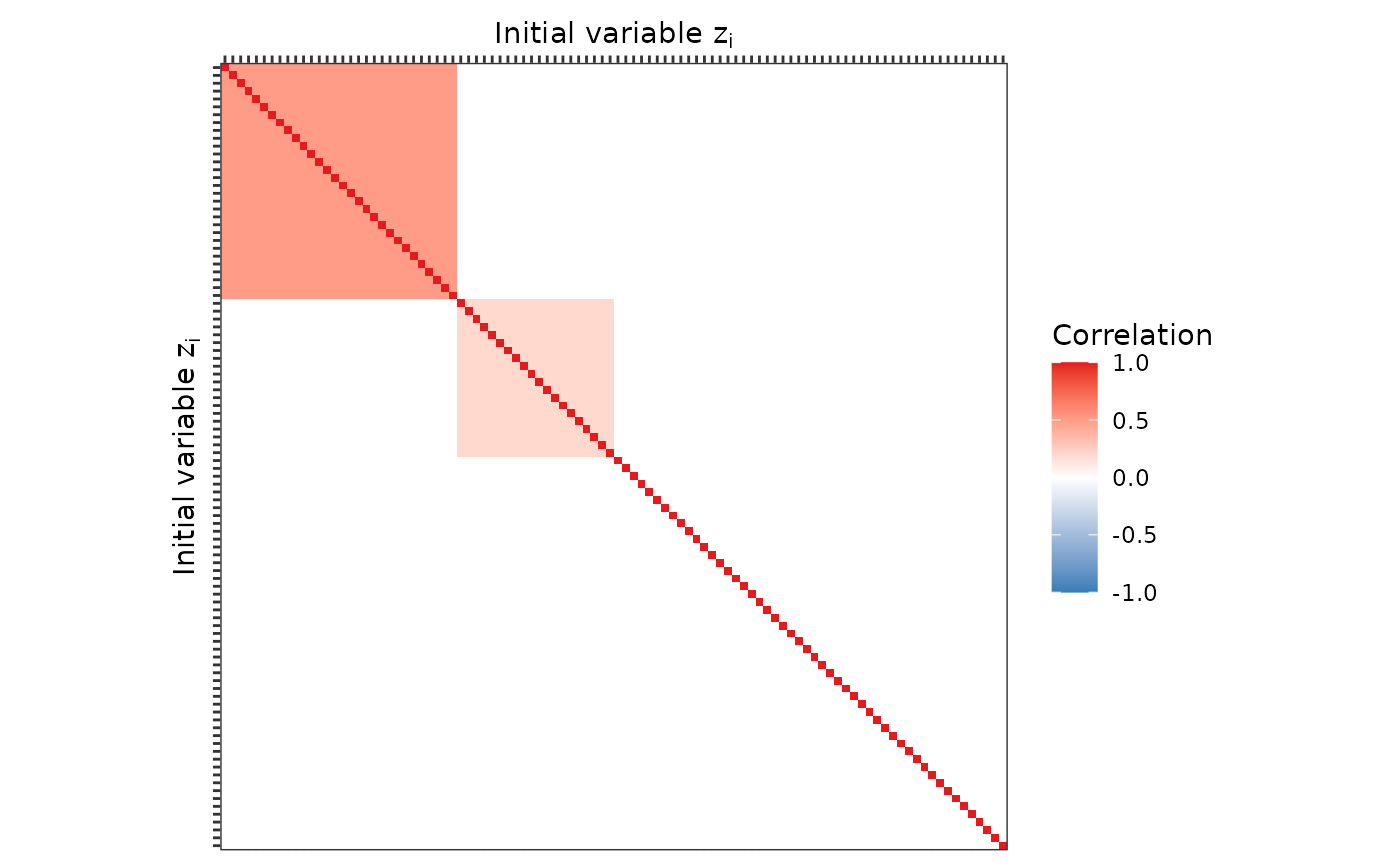
In high-dimensional simulation studies the number of simulated variables is large. We briefly demonstrate how to simulate 100 variables from a multivariate Normal distribution with block correlation matrix. This shows how to use the package functionality programmatically.

Create a block diagonal matrix easily using base::expand.grid and cor_from_upper
- Note that for 1000s of variables drawing from a single multivariate Normal distribution using mvtnorm::rmvnorm is highly inefficient and could be replaced by drawing from individual blocks of multivariate Normal distributions of smaller dimension
Transform the variables blockwise by creating a function_list from a list of functions via as_function_list
- Note the use of base::substitute to construct functions programmatically (substitute actually substitutes the passed value for i instead of the symbol i in the function definition)
- Note that the final transformation is applied to a whole submatrix at once (this is possible as long as the resulting outputs have equal number of rows)

correlation_matrix = simdata::cor_from_upper(
  100,
  entries = rbind(
    expand.grid(1:30, 1:30, 0.5), 
    expand.grid(31:50, 31:50, 0.2))
)

# create list of transformation functions programmatically
# For the first 60 variables: 
# odd varibles will be translated
# even variables will be scaled
transformation = list()
for (i in 1:60) {
  if (i %% 2) {
    transformation[[i]] = substitute(function(x) x[, i] * 5, list(i = i))
  } else transformation[[i]] = substitute(function(x) x[, i] - 10, list(i = i))
}
# the remaining are returned as they are
transformation[[61]] = function(x) x[, 61:100]
# construct single transformation function from the list
transformation = simdata::as_function_list(transformation)

# create simulation design
sim_design = simdata::simdesign_mvtnorm(
  relations = correlation_matrix, 
  transform_initial = transformation
)

We can visualise the correlation matrix as before using ggplot2.

A correlation network can often be used to clearly display such large correlation structures. To keep the network simple, we remove vertex and edge labels and adjust vertex and edge sizes.

simdata::plot_cor_network(sim_design, seed = 2,  
                          vertex_labels = NA,
                          edge_label_function = NULL,
                          edge_width_function = function(x) 0.01,
                          edge_weight_function = function(x) 0.25 * x, 
                          use_edge_weights = TRUE, 
                          edge.color = "clipped-ramp", 
                          vertex.size = 3)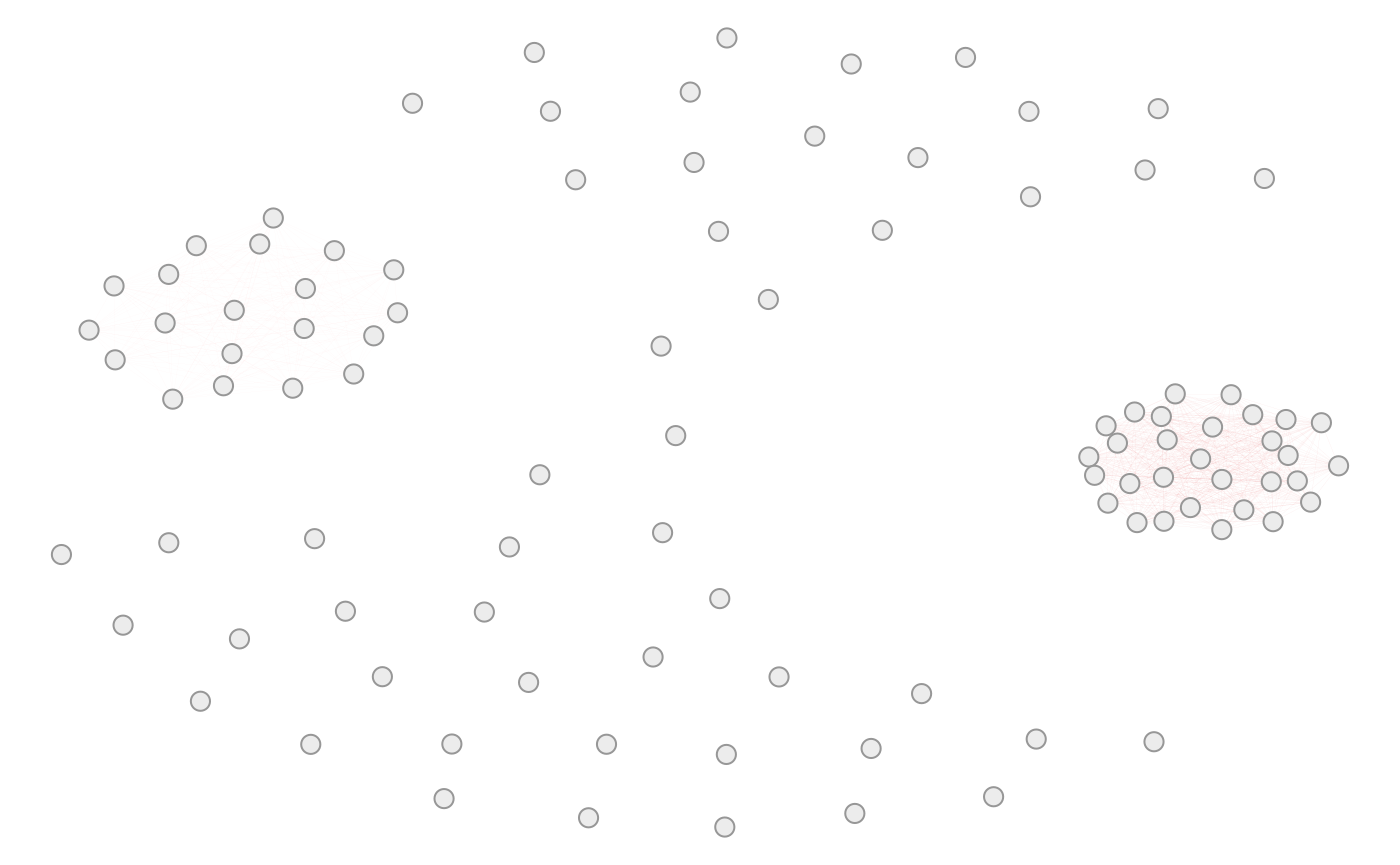

The simulated data is subsequently obtained by applying the specified transformations to the initial multivariate Normal data. It is visualised below by means of density curves for each variable (for brevity the legend is not displayed and variables are indicated by different colors).

sim_data = simdata::simulate_data(sim_design, n_obs = 50, seed = 5)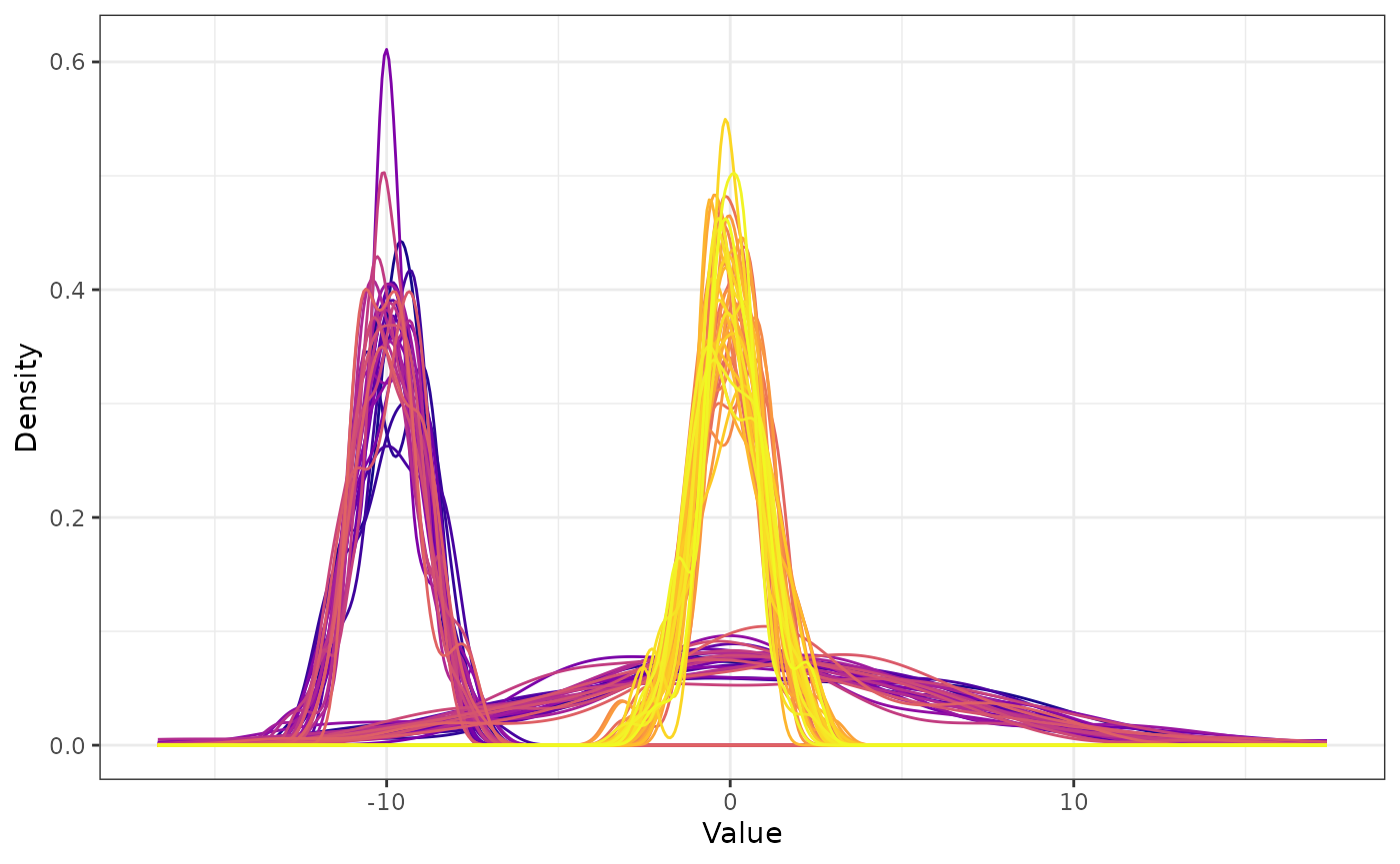

Parallelization

This example briefly shows how to use the package together with parallelization via clusters to speed up simulations. On Unix-based systems, forking provides an alternative method to parallelize code, which results in even simpler code than the one below. We use the same setup as in Example 2. The following code is not run to ensure that the vignette builds on any system, but can be used as is on any system that has the simdata package installed.

We set up a local cluster using 2 CPU threads via the parallel and doParallel packages
- Alternative parallel implementations such as future can be used.
Note that the random seed is now set via the options of doRNG in the head of the foreach loop (and NOT within the call of simulate_data).
Note that the simdata package needs to be explicitly passed to the foreach loop such that every thread has access to the library. This is Windows specific, on Unix-based systems this is not necessary as forking automatically makes the library available to all child processes.
Note that the global variable sim_design is passed to the threads automatically, but this can be forced via the .export argument in the foreach loop
The results are stored in a list.

correlation_matrix = diag(1, nrow = 5)
transformation = simdata::function_list(
    "v1" = function(x) x[, 1],
    "v2*2" = function(x) x[, 2] * 2, 
    "v3^2" = function(x) x[, 3]^2,
    "v4+v5" = function(x) x[, 4] + x[, 5], 
    check.names = FALSE # pass columnnames exactly as specified here
  )

sim_design = simdata::simdesign_mvtnorm(
  relations = correlation_matrix,
  transform_initial = transformation, 
  prefix_final = NULL
)

# parallelisation
cl = parallel::makeCluster(1)
doParallel::registerDoParallel(cl)
res = foreach(
  i = 1:10, 
  .packages = c("simdata"),
  .options.RNG = 1 # note that the seed is passed here
) %dorng% {
  simulate_data(sim_design, n_obs = 100)
  
  # do some task with the simulated data
}
parallel::stopCluster(cl)

knitr::kable(purrr::map(res[1:2], summary))

Partial functions

The simdata packages makes heavy use of function objects to define simulation designs (e.g. also NORTA based simulation). Sometimes it may be necessary to fix parameters of such functions, or define them via code. In Example 2 we created a variable v2*2 by multiplying the initial data times 2.

What if we wanted to parametrize this? If we simply use a global variable this will have undesirable consequences, as R may change the value of the global value at any time (or remove the value, which leads to a failure of the sampling procedure).

# parameter
mult = 2
transformation = simdata::function_list(
  "v1" = function(x) x[, 1] * mult # dangerous, depends on global variable!
)

sim_design = simdata::simdesign_mvtnorm(
        relations = diag(1), 
        transform_initial = transformation
)

sample1 = simdata::simulate_data(sim_design, n_obs = 5, seed = 25897165)

# change value of global variable
mult = 4
sample2 = simdata::simulate_data(sim_design, n_obs = 5, seed = 25897165)

# note the different values in both columns
knitr::kable(cbind(sample1, sample2))

v1	v1
-0.8166563	-1.633312
2.6989619	5.397924
1.2366453	2.473291
-1.1770835	-2.354167
1.9821340	3.964268

This can be avoided by the use of simdata::partial. This requires to specify the transformation as function in two parameters, of which one is fixed.

# parameter
mult = 2
transformation = simdata::function_list(
    # specify function as partial 
    "v1" = simdata::partial(function(x, mult) x[, 1] * mult, mult = mult)
)

sim_design = simdata::simdesign_mvtnorm(
        relations = diag(1), 
        transform_initial = transformation
)

sample1 = simdata::simulate_data(sim_design, n_obs = 5, seed = 25897165)

# change value of global variable
mult = 4
sample2 = simdata::simulate_data(sim_design, n_obs = 5, seed = 25897165)

# note both columns are equal now, as expected
knitr::kable(cbind(sample1, sample2))

v1	v1
-0.8166563	-0.8166563
2.6989619	2.6989619
1.2366453	1.2366453
-1.1770835	-1.1770835
1.9821340	1.9821340

simdata::partial can be used to fix an arbitrary number of parameters, and may also help if a transformation is defined inside another function (as the parameter set inside a function may not be available outside).

R session information

## R version 4.4.1 (2024-06-14)
## Platform: x86_64-pc-linux-gnu
## Running under: Ubuntu 22.04.4 LTS
## 
## Matrix products: default
## BLAS:   /usr/lib/x86_64-linux-gnu/openblas-pthread/libblas.so.3 
## LAPACK: /usr/lib/x86_64-linux-gnu/openblas-pthread/libopenblasp-r0.3.20.so;  LAPACK version 3.10.0
## 
## locale:
##  [1] LC_CTYPE=C.UTF-8       LC_NUMERIC=C           LC_TIME=C.UTF-8       
##  [4] LC_COLLATE=C.UTF-8     LC_MONETARY=C.UTF-8    LC_MESSAGES=C.UTF-8   
##  [7] LC_PAPER=C.UTF-8       LC_NAME=C              LC_ADDRESS=C          
## [10] LC_TELEPHONE=C         LC_MEASUREMENT=C.UTF-8 LC_IDENTIFICATION=C   
## 
## time zone: UTC
## tzcode source: system (glibc)
## 
## attached base packages:
## [1] parallel  stats     graphics  grDevices utils     datasets  methods  
## [8] base     
## 
## other attached packages:
##  [1] doRNG_1.8.6       rngtools_1.5.2    doParallel_1.0.17 iterators_1.0.14 
##  [5] foreach_1.5.2     knitr_1.47        GGally_2.2.1      reshape2_1.4.4   
##  [9] ggplot2_3.5.1     simdata_0.4.0    
## 
## loaded via a namespace (and not attached):
##  [1] sass_0.4.9         utf8_1.2.4         generics_0.1.3     tidyr_1.3.1       
##  [5] stringi_1.8.4      digest_0.6.36      magrittr_2.0.3     evaluate_0.24.0   
##  [9] grid_4.4.1         RColorBrewer_1.1-3 mvtnorm_1.2-5      fastmap_1.2.0     
## [13] plyr_1.8.9         jsonlite_1.8.8     purrr_1.0.2        fansi_1.0.6       
## [17] viridisLite_0.4.2  scales_1.3.0       codetools_0.2-20   textshaping_0.4.0 
## [21] jquerylib_0.1.4    cli_3.6.3          rlang_1.1.4        munsell_0.5.1     
## [25] withr_3.0.0        cachem_1.1.0       yaml_2.3.8         tools_4.4.1       
## [29] memoise_2.0.1      dplyr_1.1.4        colorspace_2.1-0   ggstats_0.6.0     
## [33] vctrs_0.6.5        R6_2.5.1           lifecycle_1.0.4    stringr_1.5.1     
## [37] fs_1.6.4           ragg_1.3.2         pkgconfig_2.0.3    desc_1.4.3        
## [41] pkgdown_2.0.9      pillar_1.9.0       bslib_0.7.0        gtable_0.3.5      
## [45] glue_1.7.0         Rcpp_1.0.12        systemfonts_1.1.0  highr_0.11        
## [49] xfun_0.45          tibble_3.2.1       tidyselect_1.2.1   farver_2.1.2      
## [53] igraph_2.0.3       htmltools_0.5.8.1  labeling_0.4.3     rmarkdown_2.27    
## [57] compiler_4.4.1

References

Binder, Harald, Willi Sauerbrei, and Patrick Royston. 2011. “Multivariable Model-Building with Continous Covariates: 1. Performance Measures and Simulation Design.” Report.

Michael Kammer

2024-07-01

Introduction

Data generation with this package

Workflow with this package

Packages used

Example 1: Independent data, no transformation

Example 2: Independent data, with transformation

Example 3: Realistic, complex data

Visualisation of initial correlation matrix

Simulation and visualisation of final data

Visualisation of estimated correlation network

Post-processing

Truncation

Standardization

Advanced simulation setup

Rejection sampling

User defined `simdesign` classes

Other initial distributions

Using real data

Aspects of high-dimensional setups

Parallelization

Partial functions

R session information

References

simdata: A package for creating simulated datasets

Michael Kammer

2024-07-01

Introduction

Data generation with this package

Workflow with this package

Packages used

Example 1: Independent data, no transformation

Example 2: Independent data, with transformation

Example 3: Realistic, complex data

Visualisation of initial correlation matrix

Simulation and visualisation of final data

Visualisation of estimated correlation network

Post-processing

Truncation

Standardization

Advanced simulation setup

Rejection sampling

User defined simdesign classes

Other initial distributions

Using real data

Aspects of high-dimensional setups

Parallelization

Partial functions

R session information

References

User defined `simdesign` classes