simdata: NORTA based simulation designs

Introduction

This document describes the workflow to define NORmal-To-Anything (NORTA) based simulation designs using the simdata package. The method is very useful to re-create existing datasets through a parametric approximation for usage in simulation studies. It is also quite easy to use, and allows the definition of presets for sharing simulation setups. General details of the methodology and further references are given in e.g. Cario and Nelson (1997) and Ghosh and Henderson (2003).

In this vignette we will prefix all relevant function calls by :: to show the package which implements the function - this is not necessary but only done for demonstration purposes.

Outline of NORTA

The goal of the NORTA procedure is to produce identically independently distributed (iid) samples from random variables with a given correlation structure (Pearson correlation matrix) and given marginal distributions, thereby e.g. approximating existing datasets.

Following Ghosh and Henderson (2003), we want to sample iid replicates of the random vector \(X = (X_1, X_2, \ldots, X_k)\). Denote by \(F_i(s) = P(X_i \leq s)\) the distribution functions (i.e. the marginal distributions) of the components of \(X\), and by \(\Sigma_X\) the \(k \times k\) correlation matrix of \(X\). Then NORTA proceeds as follows:

Generate multivariate standard normal random vectors (i.e mean 0, variance 1) \(Z = (Z_1, Z_2, \ldots, Z_k)\) with a correlation matrix \(\Sigma_Z\).
Compute the random vector \(X\) via \(X_i := F_i^{-1}(\Phi(Z_i))\), where \(\Phi\) denotes the distribution function of the standard normal distribution, and \(F_i^{-1}(t) := \inf\{x: F_i(x) \geq t\}\) is the quantile function of \(X_i\).

The resulting vector \(X\) then has the desired marginal distribution. To obtain the target correlation structure \(\Sigma_X\), the correlation matrix \(\Sigma_Z\) for the first step has to be chosen appropriately. This can be achieved via solving univariable optimisation problems for each pair of variables \(X_i\) and \(X_j\) in \(X\) and is part of the simdata package.

Caveats of NORTA

The NORTA procedure has some known limitations, which may lead to discrepancies between the target correlation structure and the correlation structure obtained from the sampling process. These are, however, partly alleviated when using existing datasets as templates, or by special techniques within simdata.

Not all combinations of given marginal distributions and target correlation are feasible by the nature of the variables. This is not an issue when an existing dataset is used as template, since that demonstrates that the combination exists.
The optimisation procedure to obtain \(\Sigma_Z\) may lead to a matrix which is not positive definite (since the optimisation is only done for pairs of variables), and therefore not a proper correlation matrix. To alleviate this, the simdata package ensures positive definiteness by using the closest positive definite matrix instead. This may lead to discrepancies between the target correlation and the achieved correlation structure.
NORTA cannot reproduce non-linear relationships between variables. This may lead to issues for continuous variables and categorical variables with more than two categories when the goal is to faithfully re-create a real dataset that features non-linear relations.
The optimisation procedure to obtain \(\Sigma_Z\) may take a while to compute when the number of variables increases. This is alleviated through the fact that this computation has to be done only a single time, during definition of the simulation design. All further simulation iterations only use the optimisation result and are therefore not subject to this issue.
When applied to an existing dataset, NORTA relies on the estimation of the target correlation matrix and marginal distributions. More complex data (e.g. special marginal distributions, complex correlation structure) therefore requires more observations for an accurate representation.

Comparison to other methods

NORTA is well suited to re-create existing datasets through an explicit parametric approximation. Similar methods exist, that achieve this through other means. A particularly interesting alternative is the generation of synthetic datasets using an approach closely related to multiple imputation, and is implemented in e.g. the synthpop R package (Nowok, Raab, and Dibben (2016)). Its’ primary aim is to achieve confidentiality by re-creating copies to be shared for existing, sensitive datasets.

In comparison, synthpop potentially offers more flexible data generation than NORTA, thereby leading to a better approximation of an original dataset. However, synthpop is also more opaque than the explicit, user defined specification of correlation and marginal distributions of NORTA. This also entails that synthpop can be generally used more like a black-box approach, which requires little user input, but is also less transparent than the manual curation of the simulation setup in NORTA. Furthermore, NORTA allows easy changes to the design to obtain a wide variety of study designs from a single template dataset, whereas synthpop is more targeted at re-creating the original dataset. Both methods therefore have their distinct usecases and complement each other.

Workflow in `simdata`

Given the outline of the method, all the user has to specify to define a NORTA design on \(k\) variables are

A \(k \times k\) target correlation matrix
The \(k\) marginal distributions for each variable, given as quantile functions

These can be estimated from existing datasets of interest. simdata offers a helper function to automate this process, but the user can also specify the required input manually. We demonstrate both use cases in the example below.

Quantile functions for some common distributions

The required marginal distributions are given as quantile functions. R provides implementations of many standard distributions which can be directly used, see the help on distributions. The quantile functions use the prefix “q”, as in e.g. qnorm or qbinom. Further implementations can be found in the packages extraDistr, actuar and many others (see https://CRAN.R-project.org/view=Distributions).

Example

In this example we will setup a NORTA based simulation design for a dataset extracted from the National Health And Nutrition Examination Survey (NHANES), accessible in R via several packages (we use the nhanesA package in this demo).

Load dataset

First we will load the dataset and extract several variables of interest, namely gender (‘Gender’), age (‘Age’), race (‘Race’), weight (‘Weight’), bmi (‘BMI’), systolic (‘BPsys’) and diastolic blood pressure (‘BPdia’). These variabes demonstrate several different kinds of distributions. For a detailed description of the data, please see the documentation at https://www.cdc.gov/nchs/nhanes.htm. Here we are not concerned with the exact codings of the variables, so we will remove labels to factor variables and work with numeric codes.

df = nhanesA::nhanes("DEMO_J") %>% 
  left_join(nhanesA::nhanes("BMX_J")) %>% 
  left_join(nhanesA::nhanes("BPX_J")) %>% 
  dplyr::select(Gender = RIAGENDR, 
                Age = RIDAGEYR, 
                Race = RIDRETH1, 
                Weight = BMXWT, 
                BMI = BMXBMI, 
                BPsys = BPXSY1, 
                BPdia = BPXDI1) %>% 
  filter(complete.cases(.)) %>% 
  filter(Age > 18) %>% 
  mutate(Gender = as.numeric(Gender), 
         Race = as.numeric(Race))

print(head(df))

##   Gender Age Race Weight  BMI BPsys BPdia
## 1      2  75    4   88.8 38.9   120    66
## 2      1  56    5   62.1 21.3   108    68
## 3      1  67    3   74.9 23.5   104    70
## 4      1  71    5   65.6 22.5   112    60
## 5      1  61    5   77.7 30.7   120    72
## 6      1  22    3   74.4 24.5   116    62

Estimate target correlation

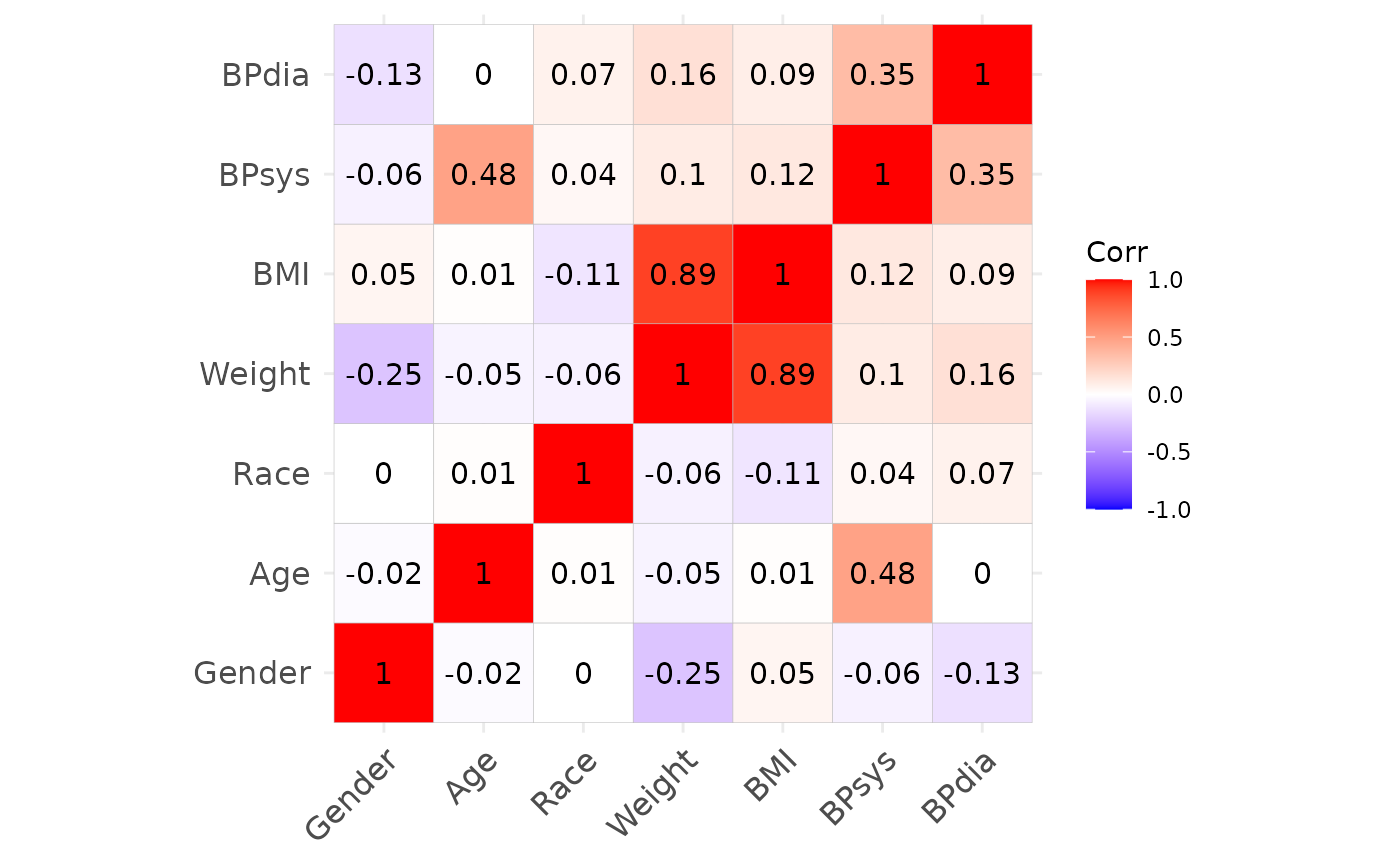
Using this dataset, we first define the target correlation cor_target and plot it.

cor_target = cor(df)
ggcorrplot::ggcorrplot(cor_target, lab = TRUE)

Define marginal distributions

Further, we define a list of marginal distributions dist representing the individual variables. Each entry of the list must be a function in one argument, defining the quantile function of the variable. The order of the entries must correspond to the order in the target correlation cor_target.

Automatically

simdata offers the helper function simdata::quantile_functions_from_data() to automate estimation of quantile functions from the available data. It does so non-parametrically and implements two approaches, one more suited for categorical data, and the other more suited to continuous data. In practice the parameter n_small can be used to determine a number of unique values required to use the latter approach, rather than the former. See the documentation for more details.

dist_auto = quantile_functions_from_data(df, n_small = 15)

Manually

We use the fitdistrplus::fitdist function to find appropriate distribution candidates and fit their parameters. Decisions regarding the fit of a distribution can be made using e.g. the Akaike information criterion (AIC) or Bayesian information criterion (BIC) displayed by the summary of the fit object returned by the function (the lower their values, the better the fit).

In case a parametric distribution doesn’t fit very well, we instead make use of a density estimate and use this to define the marginal quantile function.

Gender: a binomial distribution with \(P(2) \approx 0.5\).
Age: the distribution is not very “nice”.
- We approximate it using a kernel density estimate using the stats::density function.
- Note that the boundaries of the distribution can be more or less smoothed with the cut parameter.
- To obtain a quantile function, first we integrate the density, normalize it, and then use stats::approxfun to derive a univariable quantile function.
Race: a categorical distribution with 5 categories specified by probabilities
- Can also be implemented using the categorical distribution from the package LaplacesDemon implemented via qcat
Weight: gamma distribution parameters estimated using fitdistrplus::fitdist
BMI and systolic blood pressure: log-normal distribution parameters estimated using fitdistrplus::fitdist
Diastolic blood pressure: normal distribution parameters estimated using fitdistrplus::fitdist after removing zero values from the data

The code to implement these marginal distributions is shown below.

dist = list()

# gender
dist[["Gender"]] = function(x) qbinom(x, size = 1, prob = 0.5)

# age
dens = stats::density(df$Age, cut = 1) # cut defines how to deal with boundaries
# integrate
int_dens = cbind(Age = dens$x, cdf = cumsum(dens$y))
# normalize to obtain cumulative distribution function
int_dens[, "cdf"] = int_dens[, "cdf"] / max(int_dens[, "cdf"])
# derive quantile function
# outside the defined domain retun minimum and maximum age, respectively
dist[["Age"]] = stats::approxfun(int_dens[, "cdf"], int_dens[, "Age"], 
                          yleft = min(int_dens[, "Age"]), 
                          yright = max(int_dens[, "Age"]))

# race
dist[["Race"]] = function(x) 
    cut(x, breaks = c(0, 0.135, 0.227, 0.575, 0.806, 1), 
        labels = 1:5)

# weight
fit = fitdistrplus::fitdist(as.numeric(df$Weight), "gamma")
summary(fit)
dist[["Weight"]] = function(x) qgamma(x, shape = 14.44, rate = 0.17)

# bmi
fit = fitdistrplus::fitdist(as.numeric(df$BMI), "lnorm")
summary(fit)
dist[["BMI"]] = function(x) qlnorm(x, meanlog = 3.36, sdlog = 0.23)

# systolic blood pressure
fit = fitdistrplus::fitdist(as.numeric(df$BPsys), "lnorm")
summary(fit)
dist[["BPsys"]] = function(x) qlnorm(x, meanlog = 4.83, sdlog = 0.15)

# diastolic blood pressure
fit = fitdistrplus::fitdist(as.numeric(df %>% 
                                         filter(BPdia > 0) %>% 
                                         pull(BPdia)), "norm")
summary(fit)
dist[["BPdia"]] = function(x) qnorm(x, mean = 72.42, sd = 11.95)

What to use?

Both, the automatic and the manual way to specify marginals may be useful. The automatic way works non-parametrically which may be useful when a real dataset should be re-created, while the manual way allows to specify marginals parametrically which may be useful when the data is defined from purely theoretical specifications.

Simulate data

Now we can use simdata::simdesign_norta to obtain designs using both the manual and automated marginal specifications. After that, we simulate datasets of the same size as the original data set using simdata::simulate_data, and compare the resulting summary statistics and correlation structures.

# use automated specification
dsgn_auto = simdata::simdesign_norta(cor_target_final = cor_target, 
                                     dist = dist_auto, 
                                     transform_initial = data.frame,
                                     names_final = names(dist), 
                                     seed_initial = 1)

simdf_auto = simdata::simulate_data(dsgn_auto, nrow(df), seed = 2)

# use manual specification
dsgn = simdata::simdesign_norta(cor_target_final = cor_target, 
                                dist = dist, 
                                transform_initial = data.frame,
                                names_final = names(dist), 
                                seed_initial = 1)

simdf = simdata::simulate_data(dsgn, nrow(df), seed = 2)

Results

Summary statistics of the original and simulated datasets.

summary(df)

##      Gender           Age             Race           Weight      
##  Min.   :1.000   Min.   :19.00   Min.   :1.000   Min.   : 36.20  
##  1st Qu.:1.000   1st Qu.:34.00   1st Qu.:3.000   1st Qu.: 66.90  
##  Median :2.000   Median :52.00   Median :3.000   Median : 79.00  
##  Mean   :1.511   Mean   :50.29   Mean   :3.257   Mean   : 82.68  
##  3rd Qu.:2.000   3rd Qu.:65.00   3rd Qu.:4.000   3rd Qu.: 94.70  
##  Max.   :2.000   Max.   :80.00   Max.   :5.000   Max.   :219.60  
##       BMI            BPsys           BPdia       
##  Min.   :14.80   Min.   : 72.0   Min.   :  0.00  
##  1st Qu.:24.70   1st Qu.:112.0   1st Qu.: 64.00  
##  Median :28.50   Median :124.0   Median : 72.00  
##  Mean   :29.69   Mean   :126.2   Mean   : 71.85  
##  3rd Qu.:33.50   3rd Qu.:136.0   3rd Qu.: 80.00  
##  Max.   :84.40   Max.   :224.0   Max.   :124.00

summary(simdf_auto)

##      Gender          Age             Race           Weight      
##  Min.   :1.00   Min.   :15.99   Min.   :1.000   Min.   : 33.23  
##  1st Qu.:1.00   1st Qu.:33.91   1st Qu.:3.000   1st Qu.: 65.69  
##  Median :2.00   Median :50.65   Median :3.000   Median : 77.92  
##  Mean   :1.52   Mean   :49.82   Mean   :3.248   Mean   : 81.96  
##  3rd Qu.:2.00   3rd Qu.:64.57   3rd Qu.:4.000   3rd Qu.: 94.31  
##  Max.   :2.00   Max.   :82.89   Max.   :5.000   Max.   :221.28  
##       BMI            BPsys            BPdia       
##  Min.   :13.78   Min.   : 69.03   Min.   : -1.98  
##  1st Qu.:24.29   1st Qu.:112.23   1st Qu.: 64.11  
##  Median :28.12   Median :123.04   Median : 71.94  
##  Mean   :29.45   Mean   :126.21   Mean   : 71.65  
##  3rd Qu.:33.31   3rd Qu.:136.82   3rd Qu.: 79.66  
##  Max.   :76.55   Max.   :215.53   Max.   :124.68

summary(simdf)

##      Gender            Age             Race           Weight      
##  Min.   :0.0000   Min.   :16.00   Min.   :1.000   Min.   : 26.18  
##  1st Qu.:0.0000   1st Qu.:34.04   1st Qu.:3.000   1st Qu.: 68.51  
##  Median :1.0000   Median :50.74   Median :3.000   Median : 82.24  
##  Mean   :0.5107   Mean   :49.91   Mean   :3.263   Mean   : 84.66  
##  3rd Qu.:1.0000   3rd Qu.:64.67   3rd Qu.:4.000   3rd Qu.: 98.63  
##  Max.   :1.0000   Max.   :82.89   Max.   :5.000   Max.   :206.00  
##       BMI            BPsys            BPdia       
##  Min.   :12.44   Min.   : 64.69   Min.   : 28.25  
##  1st Qu.:24.48   1st Qu.:113.66   1st Qu.: 64.33  
##  Median :28.55   Median :125.28   Median : 72.42  
##  Mean   :29.50   Mean   :127.05   Mean   : 72.47  
##  3rd Qu.:33.61   3rd Qu.:138.92   3rd Qu.: 80.65  
##  Max.   :64.72   Max.   :204.22   Max.   :117.18

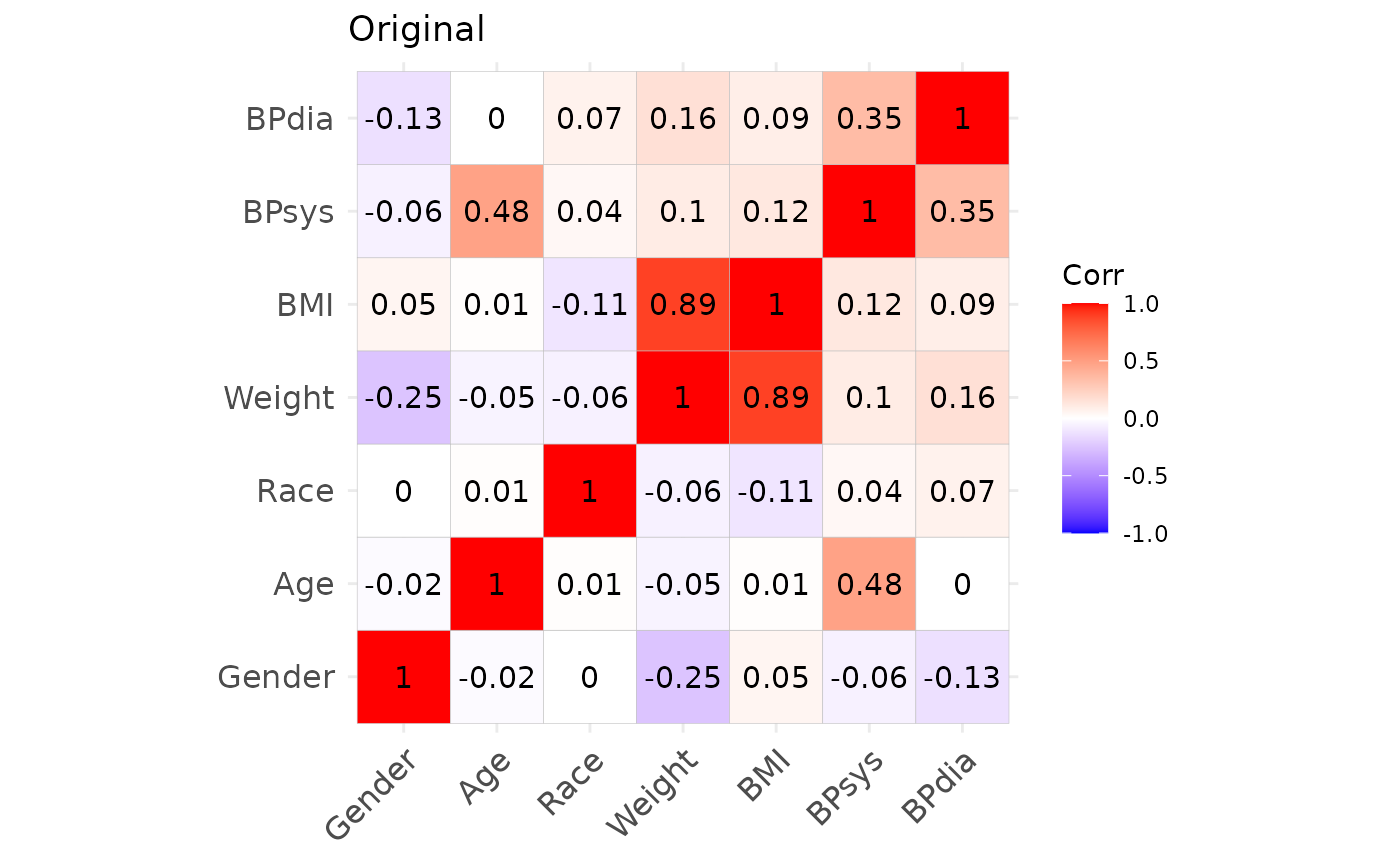
Correlation structures of the original and simulated datasets.

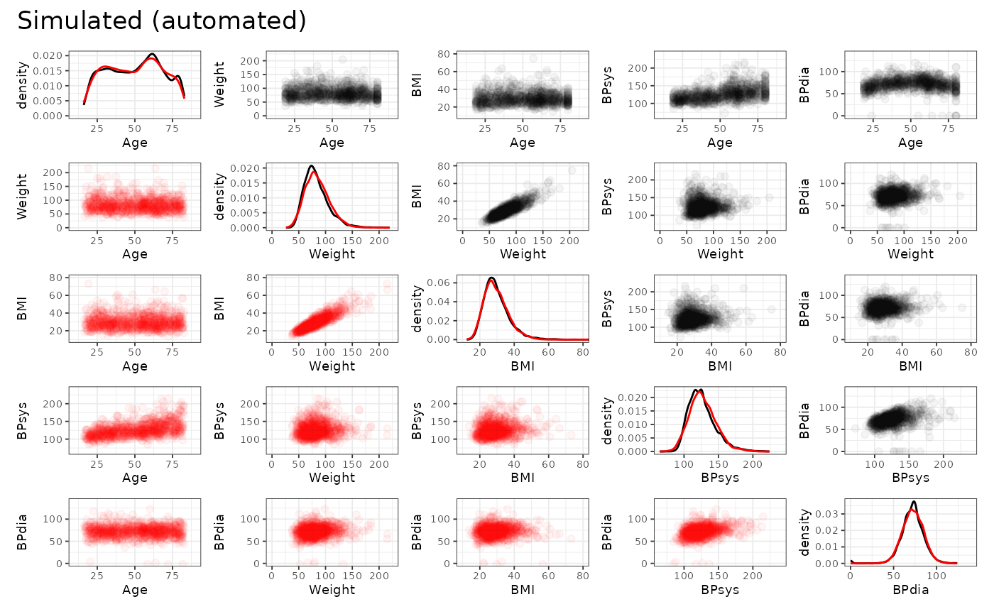
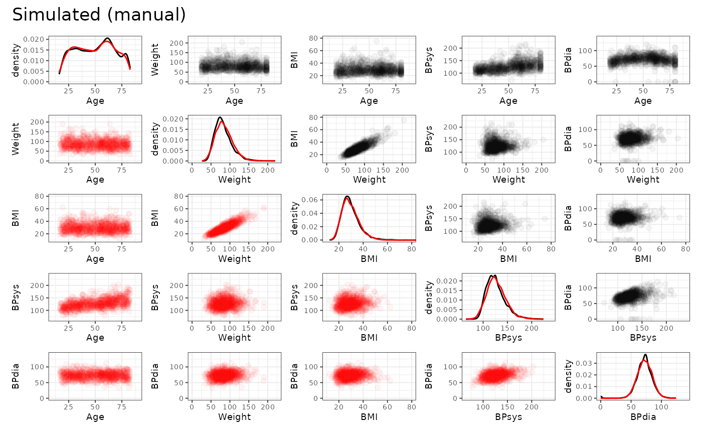
We may also inspect the continuous variables regarding their univariate and bivariate distributions. The original data is shown in black, the simulated data is shown in red. (Note that we only use the first 1000 observations to speed up the plotting.)

From this we can observe, that the agreement between the original data and the simulated data is generally quite good. Both, automated and manual specification work equally well for this dataset. Note, however, that e.g. the slightly non-linear relationship between age and diastolic blood pressure cannot be fully captured by the approach, as expected. Furthermore, the original data shows some outliers, which are also not reproducible due to the parametric nature of the NORTA procedure.

R session information

## R version 4.4.1 (2024-06-14)
## Platform: x86_64-pc-linux-gnu
## Running under: Ubuntu 22.04.4 LTS
## 
## Matrix products: default
## BLAS:   /usr/lib/x86_64-linux-gnu/openblas-pthread/libblas.so.3 
## LAPACK: /usr/lib/x86_64-linux-gnu/openblas-pthread/libopenblasp-r0.3.20.so;  LAPACK version 3.10.0
## 
## locale:
##  [1] LC_CTYPE=C.UTF-8       LC_NUMERIC=C           LC_TIME=C.UTF-8       
##  [4] LC_COLLATE=C.UTF-8     LC_MONETARY=C.UTF-8    LC_MESSAGES=C.UTF-8   
##  [7] LC_PAPER=C.UTF-8       LC_NAME=C              LC_ADDRESS=C          
## [10] LC_TELEPHONE=C         LC_MEASUREMENT=C.UTF-8 LC_IDENTIFICATION=C   
## 
## time zone: UTC
## tzcode source: system (glibc)
## 
## attached base packages:
## [1] stats     graphics  grDevices utils     datasets  methods   base     
## 
## other attached packages:
## [1] ggcorrplot_0.1.4.1  patchwork_1.2.0     ggplot2_3.5.1      
## [4] dplyr_1.1.4         fitdistrplus_1.1-11 survival_3.6-4     
## [7] MASS_7.3-60.2       nhanesA_1.1         simdata_0.4.0      
## 
## loaded via a namespace (and not attached):
##  [1] sass_0.4.9        utf8_1.2.4        generics_0.1.3    xml2_1.3.6       
##  [5] stringi_1.8.4     lattice_0.22-6    digest_0.6.36     magrittr_2.0.3   
##  [9] evaluate_0.24.0   grid_4.4.1        mvtnorm_1.2-5     fastmap_1.2.0    
## [13] plyr_1.8.9        jsonlite_1.8.8    Matrix_1.7-0      httr_1.4.7       
## [17] rvest_1.0.4       selectr_0.4-2     purrr_1.0.2       fansi_1.0.6      
## [21] scales_1.3.0      textshaping_0.4.0 jquerylib_0.1.4   cli_3.6.3        
## [25] rlang_1.1.4       munsell_0.5.1     splines_4.4.1     withr_3.0.0      
## [29] cachem_1.1.0      yaml_2.3.8        tools_4.4.1       reshape2_1.4.4   
## [33] memoise_2.0.1     colorspace_2.1-0  curl_5.2.1        vctrs_0.6.5      
## [37] R6_2.5.1          lifecycle_1.0.4   stringr_1.5.1     fs_1.6.4         
## [41] foreign_0.8-86    ragg_1.3.2        pkgconfig_2.0.3   desc_1.4.3       
## [45] pkgdown_2.0.9     bslib_0.7.0       pillar_1.9.0      gtable_0.3.5     
## [49] glue_1.7.0        Rcpp_1.0.12       systemfonts_1.1.0 highr_0.11       
## [53] xfun_0.45         tibble_3.2.1      tidyselect_1.2.1  knitr_1.47       
## [57] farver_2.1.2      htmltools_0.5.8.1 labeling_0.4.3    rmarkdown_2.27   
## [61] compiler_4.4.1

References

Cario, Marne C., and Barry L. Nelson. 1997. “Modeling and Generating Random Vectors with Arbitrary Marginal Distributions and Correlation Matrix.” Report. Northwestern University.

Ghosh, Soumyadip, and Shane G. Henderson. 2003. “Behavior of the NORTA Method for Correlated Random Vector Generation as the Dimension Increases.” ACM Trans. Model. Comput. Simul. 13 (3): 276–94. https://doi.org/10.1145/937332.937336.

Nowok, Beata, Gillian M. Raab, and Chris Dibben. 2016. “Synthpop: Bespoke Creation of Synthetic Data in r.” Journal of Statistical Software, Articles 74 (11): 1–26. https://doi.org/10.18637/jss.v074.i11.

Michael Kammer

2024-07-01

Introduction

Outline of NORTA

Caveats of NORTA

Comparison to other methods

Workflow in `simdata`

Quantile functions for some common distributions

Example

Load dataset

Estimate target correlation

Define marginal distributions

Automatically

Manually

What to use?

Simulate data

Results

R session information

References

simdata: NORTA based simulation designs

Michael Kammer

2024-07-01

Introduction

Outline of NORTA

Caveats of NORTA

Comparison to other methods

Workflow in simdata

Quantile functions for some common distributions

Example

Load dataset

Estimate target correlation

Define marginal distributions

Automatically

Manually

What to use?

Simulate data

Results

R session information

References

Workflow in `simdata`